​The Importance of the Cost of Living and Policies to Address It

The Importance of the Cost of Living and Policies to Address It

By Byron Schlomach

August 30, 2017

California is a costly place to live compared to most states. So are Massachusetts and New York. Retirees often pick up stakes and move to other states like Arizona and Florida, partly because of the warm winters, but also because the cost of living is relatively low compared to where they made their careers. Interstate cost of living differentials seem to be taken as a given, almost as natural as the different weather patterns of Oregon and Oklahoma. This study econometrically demonstrates that California is not a relatively costly place to live just because lots of people want to live there. It is a costly state due to state and local policies such as heavy-handed land-use regulation, occupational licensing, minimum wages, family and disability benefit labor regulations, and energy regulation. In other words, it is not that lots of people want to live in high-cost states and push up prices that the cost of living is high in those states. The cost of living is high because states adopt policies that make the states more costly places to do business, to buy property, and to obtain a given standard of living.

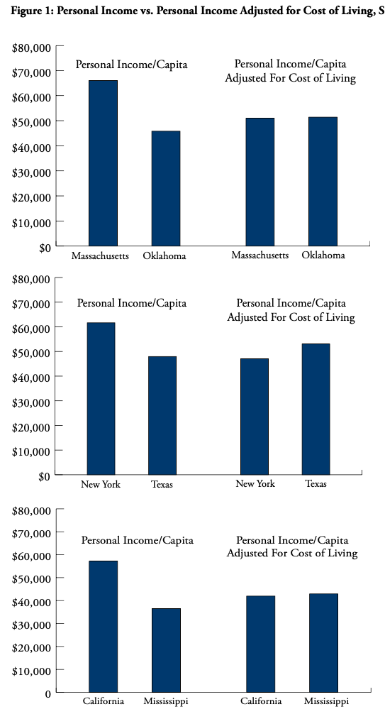
When states’ average personal incomes are adjusted for their cost of living, it radically changes the picture of which states are the most prosperous. Apparently prosperous California sinks below Mississippi. Oklahoma, middling in official statistics, rises to actually outrank Massachusetts. Texas ends up in the top 10. Apparently prosperous states that have high costs of living are shown not to be so prosperous after all, once you account for how little that can be purchased with those high incomes. And as it turns out, high-cost states tend to be “blue” in their voting patterns while low-cost states tend to be “red,” politically.

The blue-state income advantage from having more college graduates largely disappears when cost of living is taken into account. The demand for greater federal government social spending on the part of blue states is more understandable, too, when it is understood that the Federal Poverty Level of income is more limited in value in blue states than in red states. Red-state residents tend to see social programs as generous while blue-state residents see them as stingy, but the perception is less ideological than it is due to the fact that the two groups live in different cost-of-living realities. What’s more, these different realities serve to cause official statistics to overstate income inequality in the nation since individuals with relatively modest incomes often live in low-cost states where their incomes are relatively valuable.

The implications for policy are simple. First, policy makers in low-cost states should tune out interstate spending comparisons by spending advocates. Since low-cost states are often also low-spending states, government-program activists exploit this fact to advocate for greater spending. However, such comparisons are often meaningless when cost of living is taken into account, which can radically change the picture when the different spending power of dollars across states is considered. Second, state policy makers must pay much more attention to policies, such as those mentioned above, that impact the cost of living. For example, if Oklahoma reduced its licensed workforce to the national average, the resultant lower cost of living would be the equivalent of putting $800 per year into the pockets of every man, woman, and child in the state. Lowering the cost of living is equivalent to a boost in GDP, something policy makers and policy scholars have been missing for a very long time.

Introduction

Interstate differences in government spending have become part of the DNA of debates regarding expenditure levels in a number of areas including per-student spending in higher and public education, Medicaid expansion, increased funding for child welfare, and a host of other issues. As anyone who has worked with elected officials knows, advocates for such programs in low-spending states attempt to shame lawmakers into budgeting more by pointing out their states’ low spending levels compared to others.^[1] The clear implication is that lawmakers in low-spending states care less about unfortunate people than lawmakers in high-spending states. The same is true for budget decisions on issues such as teacher salaries and welfare programs.^[2]

Well-informed policymakers know that raw dollar spending comparisons across states fail to take into account an important difference among states—the cost of living. For example, most of the criticism of Mississippi for being at the bottom of the states in all manner of government-spending statistics fails to point out that Mississippi also has the lowest cost of living of all the states.^[3] Recent debates in Oklahoma regarding its 48th-ranked teacher salary status among the states fail to account for the fact that, as of this writing, only Mississippi and Arkansas have a lower cost of living than Oklahoma. Adjusting for cost of living, it turns out, can yield dramatically different results. Oklahoma’s ranking in teacher salaries, in one analysis, moved from 48th to 30th when cost of living was taken into account.

Many federal programs flow money to the states based on incomes, but incomes themselves are not the full story. A given amount of income low enough for someone to be truly in poverty in Texas is worth less in California, where the same income level makes someone absolutely destitute. Thus, were the federal government to account for cost of living, it would dramatically alter federal money flows to states. But such a change would likely ratify and reinforce poor state and local policies that lead to a higher cost of living. On the other hand, if the federal government incorporated cost of living into many of its comparative statistics, we would gain a truer picture of where we stand, not just with respect to states, but as a nation. Income inequality, for example, would likely be attenuated if income were compared after adjusting for cost of living.

Since cost of living makes a profound difference in what a dollar can buy, and this in turn makes a profound difference in a person’s well-being, it is critical we gain an understanding of what determines cost of living. In doing such an analysis, many people would likely point to population density, climate, or natural amenities that are in high demand. But an often-overlooked factor is the costs imposed by government. Government institutions such as land-use and labor regulation like a minimum wage and licensing statistically explain a great deal of the variation in cost of living across states all by themselves.

Also addressed in this paper is why state policymakers should do more to consider cost of living, and specific policies they can pursue to reduce it in their states. These include: 1) limiting land-use regulation, especially zoning, 2) reducing labor regulations, including occupational licensing, minimum wages, family leave, and disability benefit requirements, 3) passing right-to-work laws, 4) reducing startup and filing fees for businesses, and 5) reducing monopolistic regulation in electric energy.

Policy issues are often statistically investigated for how they impact GDP—either its growth over time, or its total—frequently with frustrating results. The analysis contained in this paper suggests that researchers have been missing something more fundamental: the cost of living.

Cost of Living and Personal Income

Every year, reporters and policymakers publish stories ranking states in order of economic growth, government spending, personal income, and other factors. In comparisons, it’s common to see Mississippi at the rear in many categories, especially income. Despite its growing and dynamic economy, Texas seems doomed to be stuck in the middle. Oklahoma often falls below Texas in various measures. Meanwhile, northeastern states such as Massachusetts and New York are firmly in command at the top. This pattern is exhibited in federal personal income statistics, which are often popularized in various rankings and comparisons of states.^[4] Table 1 shows per capita personal income (personal income per person) numbers for all the states and Washington, D.C.

Of the top 10 states (and the District of Columbia) in personal income per capita, seven are in the Northeast. The District ranks at the very top, and the top 10 are rounded out by California, Alaska, and Wyoming. Oklahoma and its neighbors are mostly in the bottom half of states, with Colorado ranked highest. Mississippi, as usual, brings up the rear behind New Mexico and West Virginia. Many view a ranking like that in Table 1 as indicative of well-being, implying that the Northeast and California have come out on top, Texas has a long way to go yet, and places such as West Virginia and Mississippi are suffering.

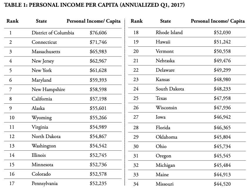
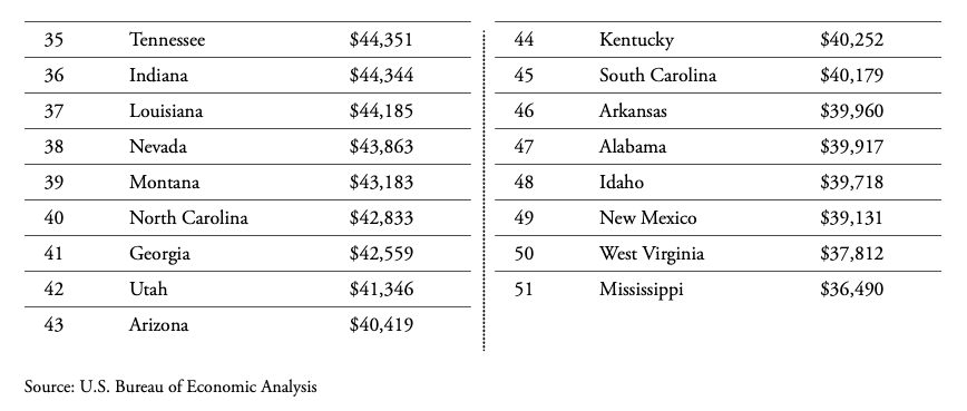
One problem with Table 1 and the conclusions that naturally arise is that a dollar spent in Boston does not buy as much as a dollar spent in Fort Worth, Oklahoma City, or Birmingham. More than a few southerners have been lured to the Northeast by large salaries only to find out the cost of living, especially in housing, is nothing like where they grew up. This is a major reason cost-of-living calculators have become popular on the internet.^[5]

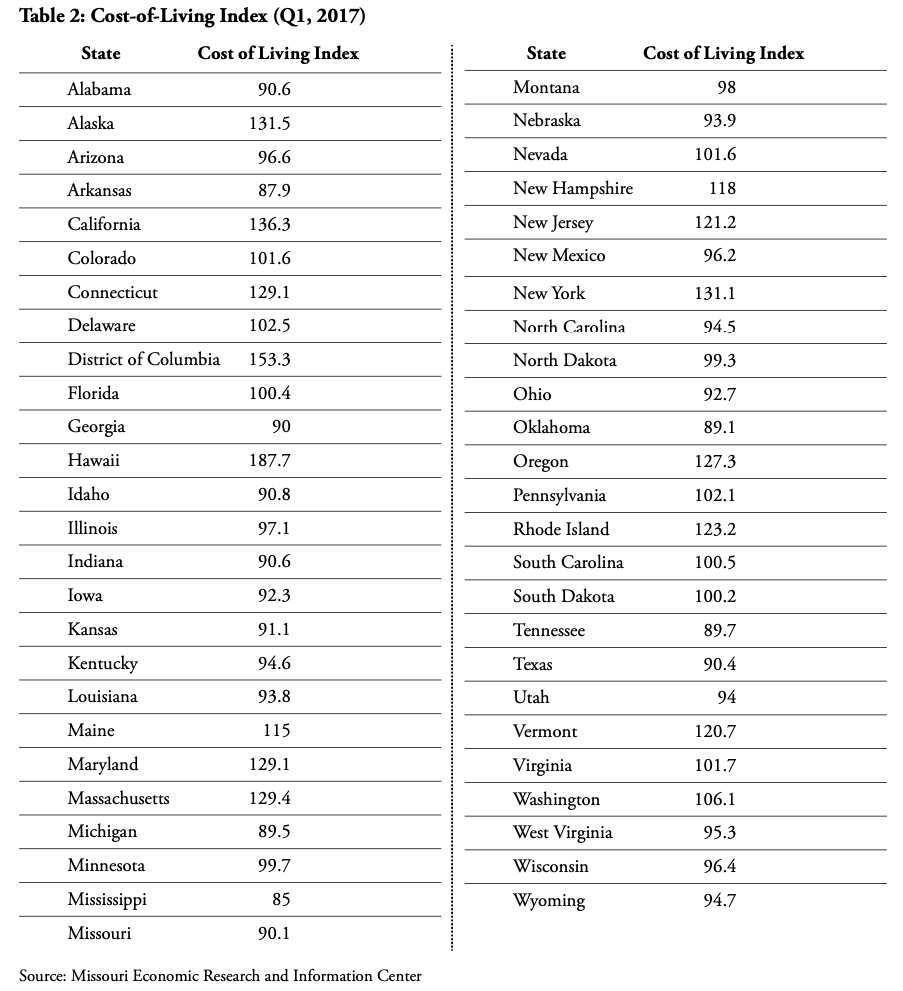
Table 2 shows an index for cost of living across the states. This index, centered on 100, gives relative cost-of-living levels for each state. The higher the index number, the greater the cost of living. This allows for state-to-state comparisons. For example, Alaska’s cost of living, with an index value of 131.5, is 45 percent higher than Alabama’s at 90.6. That means it would require $145 in Alaska for a person to possess the same purchasing power as $100 in Alabama. Hawaii’s cost of living (187.7 index value) is more than twice that of Mississippi’s (85 index value). Thus, it is misleading to judge well-being across states by simply referencing the statistics in Table 1. What’s more, there is a strong correlation between cost of living and per capita personal income. A comparison of Tables 1 and 2 yields a correlation coefficient of 0.65. This means that when cost of living is higher in one state than in another, it is very likely that personal income will be too. This is no surprise since these two factors impact each other. Income needs to be higher when cost of living is higher in order to cope with the circumstances. But higher incomes also tend to yield a higher cost of living because incomes are a business expense.

A couple of quick remarks on cost-of-living indexes is warranted at this point. First, the index in Table 2 does not rely on federal data. It relies, instead, on data produced by a private company, C2ER, which sells its data on a subscription basis. The Missouri Economic Research and Information Center uses the C2ER data to create its own proprietary index. Like federal data, C2ER apparently heavily relies on urban data. Second, a valid criticism of any index, including those used to statistically investigate cost-of-living variations later in this paper, is that their values depend heavily on judgment calls by those who put them together. For example, different prices of goods and services are given different weights depending on how significant they are in peoples’ budgets. These weights do not necessarily match the consumption patterns of a particular individual—patterns as varied as the number of individuals. Nonetheless, indexes likely contribute to our overall knowledge and can lead us to ask relevant questions about policy decisions.^[6]

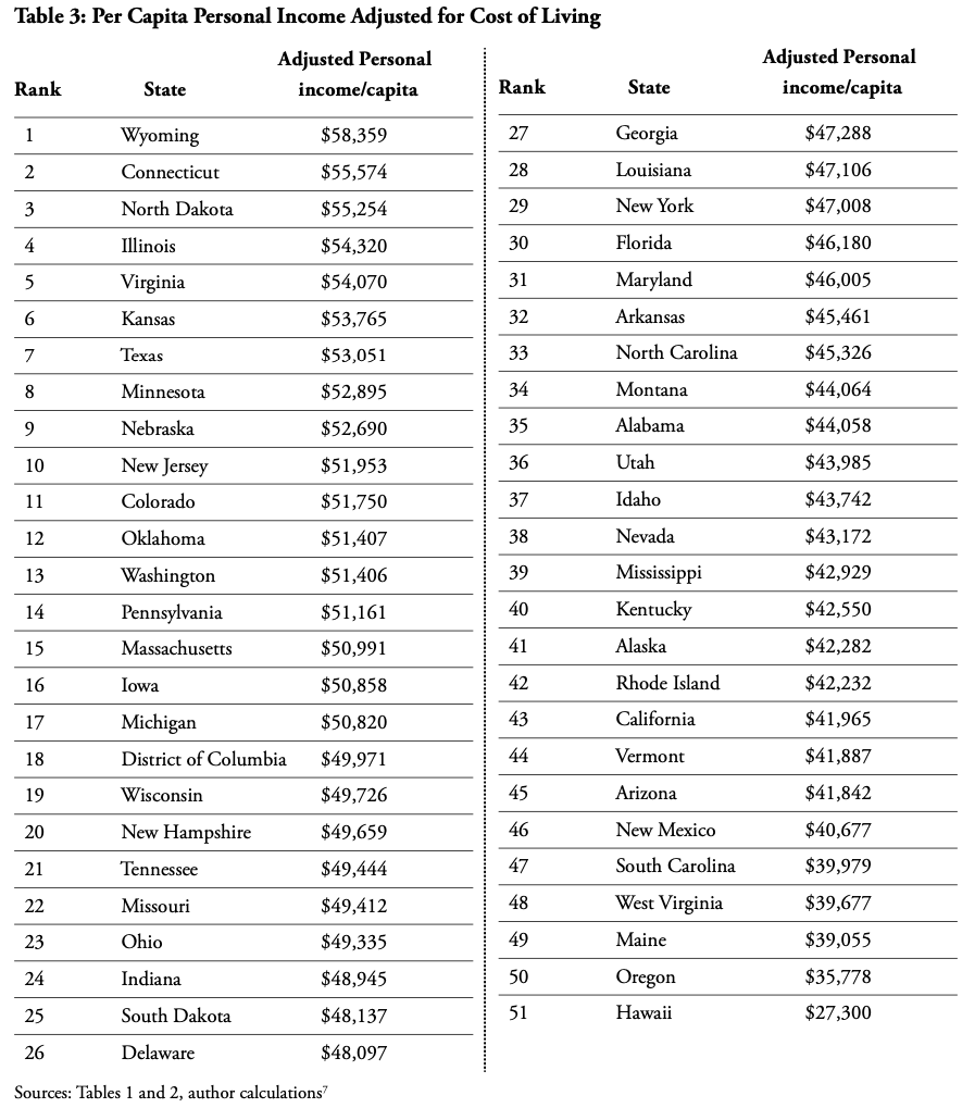
To avoid having people misled by raw per capita personal income statistics, the numbers in Table 1 need adjusting to account for the cost of living. Using the index values in Table 2, the per capita personal income of each state can be deflated or inflated to equate the relative purchasing power of dollars across states. In states with index values lower than 100, purchasing power is relatively high, so their income numbers will inflate when adjusted. States with high costs of living will see their income numbers decline when adjusted so as to reflect the fact that dollars in those states do not stretch as far. (An endnote illustrates how this simple calculation is done.) The result is Table 3, whose dollar values can be used as a means of comparison of the relative purchasing power of the states’ actual per capita personal incomes.

Sources: Tables 1 and 2, author calculations^[7]

Note that once states’ per capita personal incomes are adjusted for cost of living to reflect purchasing power, the rankings radically change. Only two northeastern states, Connecticut and New Jersey, remain in the top 10. Formerly middle-ranked Texas jumps 18 spots to number 7.

lower cost of living. Oklahoma, once ranked 29th and 13 spots behind Colorado, rises to 12th, just behind Colorado. Oklahoma outranks Massachusetts, which had ranked third. California drops to 43rd, behind Mississippi’s 39th. Hawaii now takes the bottom spot, and a distant bottom at that. Figure 1 shows how the fortunes of different states change depending on whether or not personal income is adjusted for cost of living.

Implications from Cost-of-Living Adjustments

Place Greater Emphasis on Cost of Living

Policymakers, policy analysts, and lobbyists, especially on the conservative side, tend to emphasize economic growth—enhancing gross domestic product—over just about anything else as an end to be achieved in making policy. However, it is clear that cost of living matters a great deal. While it appears that Mississippi is a permanent economic bottom dweller among the states, the reality is that once cost of living is taken into account, it would take years of stronger-than-average economic growth for Hawaii to catch up with the next state above it, and decades for it to catch up to Wyoming, once cost of living is taken into account. The Northeast, truly an economic engine if for no other reason than its population density, is much less prosperous than it otherwise appears when cost of living is included in comparisons.

The importance of cost-of-living in determining the true value of income shows why policymakers should not single-mindedly pursue policies that appear to achieve greater economic growth, but should also work toward a lower cost of living. After all, reducing the cost of living by 10 percent has the same impact on people’s standard of living as a 10 percent increase in their incomes.

Economic growth across the states varies a great deal over time. Highly regulated states often grow robustly. During the last recession and its slow recovery, relatively lightly regulated Texas was the growth state many pointed to. More recently, California has done relatively well. Much of the cycling of economic growth through the states occurs due to the waxing and waning of dominant industries. When oil is doing well, Alaska, Wyoming, Texas, and Oklahoma do well. When tech is doing well, so does California and Massachusetts. When real estate is doing well, so does Arizona. Many of the economic forces that determine which states are doing well are international in scope and largely outside the control of state policymakers. The evidence described below, however, indicates that cost of living is substantially influenced by state and local policies.

Low Personal Income States Should Not Mimic High Personal Income States

Cost of living makes many comparisons of well-being across states much less meaningful. A 2012 article in Time entitled “Blue States Barack Obama Won In 2012 Are More Educated Than Red States” is a case in point.^[8] Blue states tend to have relatively high personal income levels, so the relationship expressed in the Time article is true. But it is not quite so true when we account for purchasing power.

A simple single-variable linear regression, a mathematical method that measures the relationship between variables, shows that a one-point increase in the percentage of a state’s population with a bachelor’s degree is associated with a $1,217 increase in per capita personal income (appendix, Table 7). However, if we use the same technique but replace personal income with per capita personal income adjusted for cost of living, there is a much different result. A one-point increase in a state population’s share with a bachelor’s degree is associated with a relatively modest rise in purchasing power of $286. What’s more, of the two regressions, the latter—which uses the better measure of well-being, personal income adjusted for cost of living—suggests there might be no relationship between average well-being in a state and the percentage of the population with college degrees after all(see Appendix). The seeming advantage that states with more college graduates appear to have is drowned out by their high cost of living.

The cost of living also renders many interstate spending comparisons meaningless, especially when the spending is mostly on salaries. Public education, where most of the emphasis is on salaries, particularly comes to mind. In straight comparisons across states, Oklahoma, for example, ranks 48th among the states in teacher pay, but when cost of living is taken into account, it ranks 30th.^[9] Mississippi’s seeming bottom-dwelling status in all measures related to dollars changes considerably when cost of living is taken into account, just as it did in Table 3 above as compared to Table 1.

Activists pushing for higher spending on various programs in low-spending states often claim that differences in income are attributable to differences in state spending. The analysis in this paper (below) suggests that the causal flow is different: state regulations, which push up the cost of living, force those with modest incomes to migrate to lower-cost states, leaving behind those with higher incomes—and college degrees—who can afford the higher prices of everything, including government services (and taxes).

Higher spending on government in high-cost states may or may not buy more government goods and services. It depends on the specific price circumstances in the various states. Often, activists in low-spending states point to the high spending of other states policies in areas like education, transportation, the arts, entertainment, parks, and other government-financed amenities, and insist that their states follow suit. This analysis suggests that much of the high spending in some states is only compensating for higher prices and does not necessarily result in more services. Besides, many low-spending states like Oklahoma and Texas are actually better off than high spenders like California and Massachusetts, although this is only apparent after accounting for cost of living.

Red States/Blue States, Federal Programs, and Poverty Definitions

Writers highlighting the differences between “red” and “blue” states note that blue states, which tend to be northeastern, west coastal, and urban, have higher incomes. Blue states, on average, see their residents attain higher levels of education. Blue states also receive less from the federal government in comparison to what they pay in federal taxes.^[10] What is often overlooked, however, is that northeastern and West Coast states (and the District of Columbia) also have higher costs of living. That factor changes the resulting picture considerably. Red states, which vote for (professed) small-government conservatives, are often criticized over the fact they receive more federal money compared to what they pay in taxes than blue states. It turns out the difference in cost of living between the two sets of states has more to do with this than any seeming hypocrisy on the part of red state voters.

Federal entitlement money that flows to the states is driven by the federal poverty level (FPL), a level of income used to determine eligibility for many programs, including school lunches, Temporary Assistance to Needy Families, and Medicaid. The FPL for a family of four in the lower 48 states is $24,600, regardless of whether that family lives in San Francisco, New York City, Oklahoma City, or Fort Worth. In Alaska the FPL for a family of four is $30,700 while in Hawaii it is $28,290.^[11] Presumably, these two states get a bump due to the higher cost of living, but if this is the case, Hawaii should receive a greater bump than Alaska, according to Table 2.

Table 4 shows the four-person family FPL for each state adjusted for that state’s cost of living or purchasing power. The average of these values for Washington, D.C., and the 20 blue states that voted for Hillary Clinton in 2016 is $21,078; they have a relatively high cost of living and the lower number reflects the fact that $24,600 buys less than in other states. The average for the 30 red states that voted for Donald Trump, with their lower cost of living, is 24 percent higher, at $26,239. Even though Alaska’s FPL is the highest of the states, the purchasing power of the FPL in Alabama is 16 percent higher due to that state’s much lower cost of living. Mississippi’s FPL purchasing power is 60 percent higher than that of California due to the difference in the cost of living between the two states.

 

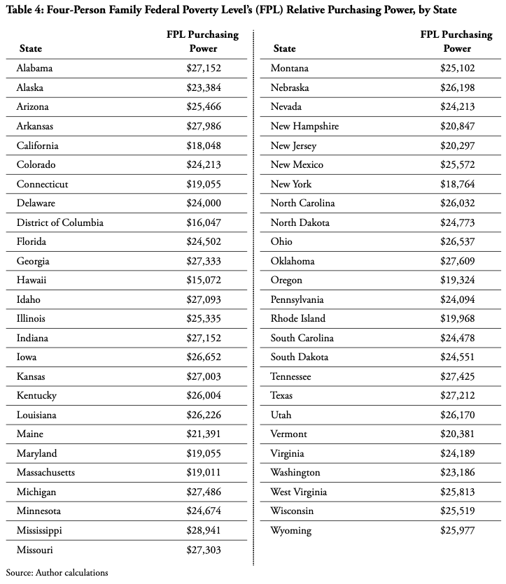
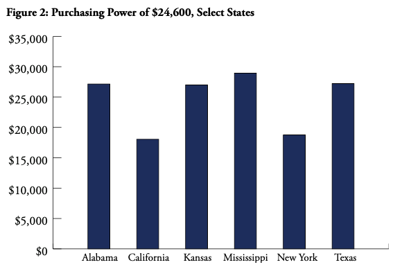
Table 4 looks at the relative purchasing power of the FPL for a family of four in each state. The dollar levels serve as a common metric for comparing the purchasing power of actual FPL dollar amounts (a uniform amount for all states except Hawaii and Alaska). Table 5 represents a different view. Suppose $24,600 is the “right” amount as the FPL for a family of four in South Carolina where the cost-of-living index value is near 100. Table 5 reflects the amount of actual dollars a family of four would need in each state to buy the same amount of stuff that $24,600 can buy in South Carolina. It also shows the difference between these constant-purchasing-power dollar amounts in each state and the actual FPL in each state.

 

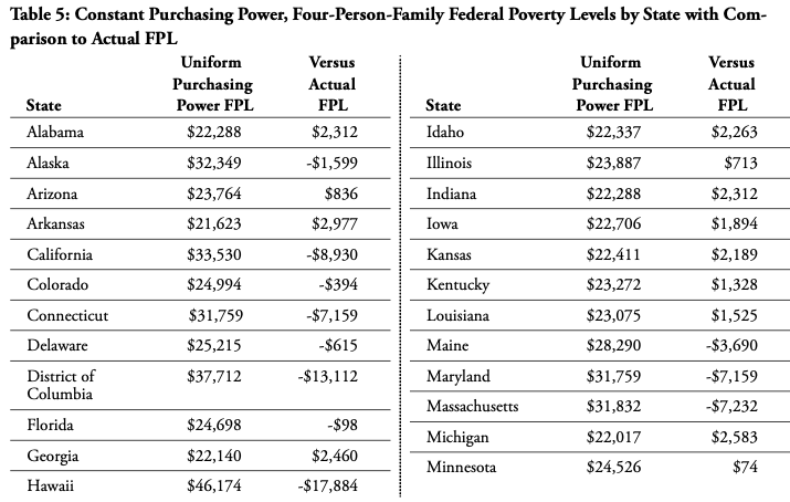
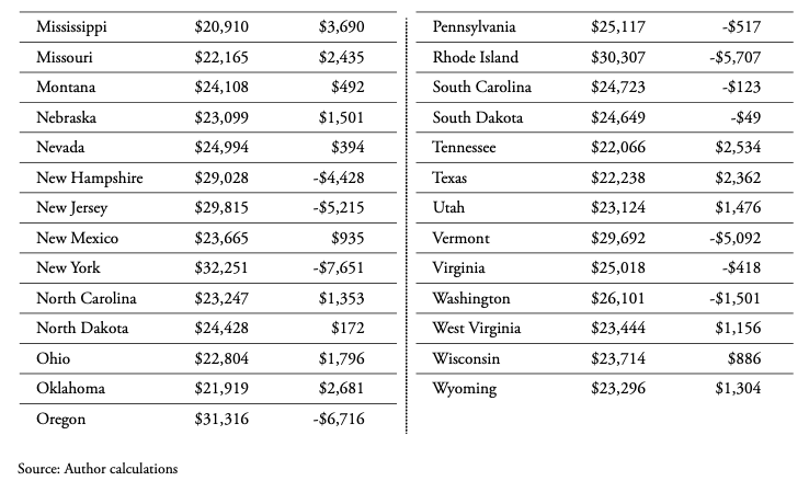
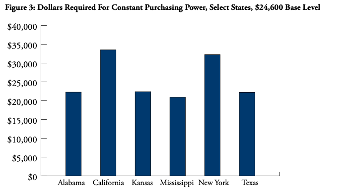
With $24,600 as the base for the calculation (including for Hawaii and Alaska), states with a high cost of living require more than $24,600 to keep purchasing power constant, while states with a low cost of living require less. Blue states in the last presidential election have an average constant-purchasing-power FPL from Table 5 of $29,613. The red-state average is $23,334. For blue states, the actual federal FPL averages $4,837 too low in comparison to Table 5 values. In red states, the $24,600 poverty level income is too high by an average of $1,417.^[12]

In high-cost blue states like Hawaii, California, New York, and Massachusetts, where the FPL seems too low, it would not be surprising that many perceive federal eligibility guidelines for assistance programs to be parsimonious. People in Connecticut know how little $31,000 can actually buy in that state. To them and those in other high-cost states, $24,600 for a family of four is a pittance. In Mississippi, though, $24,600 is quite a bit more than a pittance. People in relatively low-cost red states may consider the FPL to be overly generous, while in high-cost blue states, the same FPL appears stingy. Both perceptions, which appear to be based on regional differences in ideology, can be based on the facts of local circumstances. Residents of blue states and red states live in different cost-of-living realities.

These different realities have translated into states’ policies. For example, due to the Supreme Court’s decision, states may choose whether or not to expand Medicaid programs under the Affordable Care Act. Nineteen states have opted not to do so as of this writing, only two of which are blue states, the others having, for the most part, a low cost of living. Many federal programs, in fact, involve state and federal cost sharing with states allowed some level of discretion as to the degree of participation. One would expect states with higher per capita incomes to receive less federal money compared to taxes paid than states with lower per capita incomes. In fact, this is true, and it translates into a red state/blue state dichotomy.

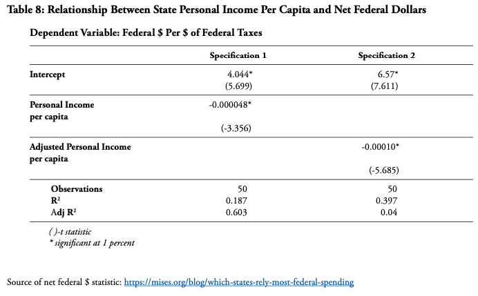
When the relationship between per capita personal income and federal dollars received per dollar paid in federal taxes is statistically tested (appendix, Table 8), there is, indeed, a negative relationship. That is, higher income for a state is associated with fewer federal dollars. However, this statistical relationship was not particularly strong. The statistical relationship between per capita personal income adjusted for cost of living is actually much stronger. This suggests that states and the federal government are pursuing policies that, however imperfectly, adjust significantly to differences in the cost of living.

The fact that states have, to the degree allowed, adjusted their policies to cost of living under federal programs illustrates the power of federalism. From its remote enclaves in Washington, D.C., the federal government does not need to determine a uniform standard of nominal spending in any area on the part of states, nor should it. Local circumstances should have the control, and those circumstances determine policy outcomes, not universal spending dictates from Washington. Obamacare’s Medicaid expansion mandate was particularly inappropriate for low-cost states, and they have acted accordingly, often refusing to expand.

We often see the red state/blue state dynamic playing the same tune in different ways. On one hand, the federal government accidentally treats red states relatively generously due to their low cost of living and apparent lower incomes. For red states, this comes at some cost since many federal programs require state matching funds. Red states’ budgets, more tuned to actual state-level needs, are at risk of federal priorities becoming a dominant budgeting consideration. On the other hand, blue states, accidentally treated less generously by the federal government due to their high cost of living and apparent higher incomes, push for federal program expansion that is unsuited for and unwanted by red states. Red states perceive federal largesse as threatening to their fiscal situations, while blue states hardly see it as largesse at all.

This discussion raises a question. Shouldn’t the federal government adjust the FPL for each state just as it already does for Alaska and Hawaii, perhaps more along the lines of that in Table 5? If the federal government made such a change in policy, the highest FPLs would mostly occur in northeastern and West Coast states and lower FPLs in southern and midwestern states. This is logical if policy is aimed at maintaining a certain minimum standard of living, which clearly costs different amounts of money from state to state.

The idea of varying the FPL according to a state’s cost of living seems to make a great deal of sense, but there are two issues that should be considered. First, as noted above, states and the federal government are already adjusting to cost of living to some degree. High-cost (blue) states already tend to be more generous in expanding programs where the federal government allows for discretion and cost-shares with states. Perhaps a better policy would be for the federal government to allow for even greater flexibility and cost-share over a greater range of program parameters.

Second, as explained below, cost of living appears to be related to state and local regulations and institutions. If the statistical analysis accurately reflects policies’ impact on the cost of living, having the federal government adjust FPL for each state’s cost of living would effectively ratify what are arguably costly and foolish policy decisions made at the state and local levels. To the extent that there is unfairness inherent in federal social programs as a result of failing to account for cost of living, this might be mostly attributable to costly state and local policies. There is no sound ethical or policy justification for having the federal government support unwise decision-making by states while effectively penalizing good decisions. Instead, lawmakers in high-cost states should pursue policies to reduce the cost of living. The ball is in their court, not that of Congress.

Income Inequality

One last issue arises from addressing cost of living: income inequality. This has become a central motivating issue in recent years, thanks largely to the writings of Thomas Piketty,^[13] Paul Krugman,^[14] and Robert Reich.^[15] However, the current level of income inequality in the United States is exaggerated and misstated by official statistics that fail to take cost of living into account. The apparently highest-income states, for the most part, are not the highest-purchasing-power states. That is, personal income unadjusted for cost of living does not reflect how well or poorly people actually live. If the individual incomes were adjusted for cost of living (purchasing power) the lion’s share of low-income individuals would likely find their purchasing power enhanced relative to income while most high-income individuals would find their purchasing power discounted. Just exactly how adjusting for cost of living would impact inequality measures is not known, but the likelihood is that incomes adjusted for cost of living (purchasing power) would be significantly more equal compared to current measures.^[16] And in fact, research published by the Texas Public Policy regarding how many individuals would be considered in poverty in various states if cost of living were taken into account is strong evidence that inequality would be attenuated if income were adjusted for cost of living.^[17]

Given the apparent rise in income inequality in recent years, a good question for further research is whether states have increasingly diverged in their cost of living in recent decades as income inequality has increased. However, the types of regulation that have pushed up the cost of living in many states are relatively new. Zoning, which is associated with a higher cost of living, is about 100 hundred years old, but its spread was slow and gradual. Right-to-work legislation, strongly associated with a lower cost of living in the analysis below, spread geographically first in the South, where incomes have historically been low. Circumstantial evidence appears to match policies that diverge with the cost of living across states with the changes in income inequality. Nothing has been done here to tease out the relative influences of different potential causes of inequality in the United States, but those who seek to make it an issue have an obligation to do so.

Why the Differences in Cost of Living?

Some might object to the cost-of-living-adjusted rankings in Table 3 on the grounds that many things people value in different states is left out of a dollar number. Hawaii, for example, has a wonderful climate, scenic vistas, and year-round outdoor activities. California has its beautiful coast. Northeastern states have many cultural amenities, rich histories, and readily available goods and services due to high population densities. All of these intangibles have a real impact on people’s standards of living but cannot be easily boiled down to a dollar value.

Intangibles certainly make a difference and can help to explain the differences in the cost of living to some extent. Economists do try to measure the value of intangibles using statistics and calculating what economists call hedonic prices.^[18] However, even if a true measure of relative well-being lies somewhere between Tables 1 and 3, there is currently no way to know where exactly it does lie.

One explanation for the high cost of living in Hawaii and Alaska is their remoteness. Neither state is self-sufficient in modern amenities, so they require long supply chains. However, bulk water transport is the cheapest form of transportation, so it is not obvious that remoteness explains anything. And as Table 6 illustrates, states that are similar and abut each other can have significantly different cost-of-living levels. For example, Washington, D.C.’s cost of living is 19 percent higher than Maryland’s and 50 percent higher than Virginia’s. New York’s is 8 percent higher than New Jersey’s, and Virginia’s is 7 percent higher than West Virginia’s, the latter being The Mountain State, where cost of living would be expected to be relatively high. None of these significant differences can be attributed to intangible amenities or costly supply chains.

 

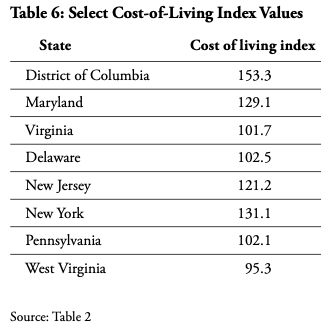
Where, then, do these differences come from? Researchers have looked into different explanations for variations in the cost of living. The analysis in this paper (below) is mainly concerned with how public policies impact cost of living, but others have focused mainly on geography and other variables largely out of the control of policymakers. One 1979 study looked at the cost of living across metropolitan areas and concluded that the major factors associated with a higher cost of living were cold climates and metropolitan population size.^[19] Another study looked at cross-state cost-of-living differences and identified per capita income, the unemployment rate, state geographic area, average annual heating degree days, amount of a state’s coastal area, the amount of toxic releases into the environment, and whether a state has a right-to-work provision.^[20] The same authors (Cebula and Toma) found similar associations with differences in the cost of housing across states in 2006.^[21]

Policies That Impact the Cost of Living and What to Do About Them

As it turns out, much of the variation in cost of living across states can be attributed to one costly phenomenon: government. This is evidenced by the statistical relationships that were tested between cost of living and policy variables explored in The 50-State Small Business Regulation Index, written by economist Wayne Winegarden and published by the Pacific Research Institute in 2015.^[22] This publication separately ranks the states according to 14 regulatory and institutional variables to determine an overall ranking. Several of these variables are indices devised to measure the relative severity of various state policies within specific policy areas as objectively as possible.^[23]

The relationship between cost of living and the various regulatory variables explored by Winegarden was analyzed using linear regression, a statistical technique. Full results are reported in the appendix (Table 9 and subsequent tables). The third-quarter 2015 index values from the Missouri Economic Research and Information Center, rather than the more recent values in Table 2, were used in the statistical analysis due to the time proximity to Winegarden’s referenced measures. Detailed results are in the appendix, but only general results and some policy judgments will be discussed here.^[24]

One technical note: Policy variables alone mathematically explain 64 to 73 percent of the variation in cost of living across states. This is a strong result from a purely statistical point of view. The policy variables come from a variety of sources and, where they are indices, have been developed independently of each other. Other sources of policy variables could have been used, such as various economic freedom indexes, but these sources consist of a high number of sub-indexes often all developed by the same researchers.

To summarize the results, the following factors are associated with higher costs of living: strict zoning laws, no state right-to-work law, a state disability insurance requirement, higher occupational licensing requirements, enhanced state family leave requirements, a higher state minimum wage, higher fees and filing costs for new businesses, and greater electric energy regulation. To some extent, it would be expected that anything that regulates real estate would show significant results in a statistical analysis of cost of living, since housing generally gets heavily weighted due to its significance in people’s budgets. But the other results described below give a good indication of where policy should move in reducing the cost of living. It is not all about land or housing regulation.

Each of Winegarden’s policy variables that are statistically related and likely determinative of the cost of living is described below with specific policy suggestions that arise from the statistical analysis. For information on Winegarden’s policy variables that were found to be statistically unrelated to cost of living, see the appendix.

Land-Use Regulation

The index used in this analysis is the Wharton Residential Land Use Regulatory Index, which indexes zoning regulation as standard deviations from a mean value set at zero. Values of the index run from -1.13 for Kansas to 2.32 for Hawaii.^[25] The greater the regulation, the greater the value of the index. Mostly, the overall issue rated in the index is zoning, with all its regulatory constructs such as setback requirements and waiting times for variances. Zoning makes land more expensive by creating artificial scarcities and regulatory hoops, adding to the cost of living. Therefore, one would see a positive relationship between this index and a cost-of-living index. And the analysis indicates that an increase in a state’s zoning regulation is associated with an increase in its cost-of-living index value.

The results reported here might partly arise from regulations at the local level that are often coincident with zoning as well as the zoning itself. For example, a recent report from the National Association of Home Builders showed nearly a 30 percent increase in costs to comply with regulations in just the past five years. From April 2011 to March 2016, it was estimated that average regulatory costs in a home built for sale rose from $65,244 to $84,671.^[26] All of these facts comport with a recent federal ruling in which local regulation in San Francisco was recognized as causing “the limited supply—and correspondingly high price—of rental units in San Francisco.”^[27]

Policy Recommendations:

Limit Local Land Regulation, Especially Zoning

The analysis strongly suggests that lawmakers should take steps to curb the power of local governments to regulate land development. Local policymakers are often pushed into counterproductive policies by vocal interests of various sorts, not the least of which are residents who want to control their environment beyond the confines of their own property.^[28] Zoning, construction regulations have made it harder to develop property and provide housing close to the cost of actual construction. As Randal O’Toole of the Cato Institute has pointed out, differences in the price of housing across the country are directly and positively related to artificial land scarcities caused by a variety of land-use regulations, including zoning.^[29]

If state legislatures are serious about lowering the cost of housing—a major factor in cost of living—they should prohibit local governments from regulating lot sizes and architectural styles, and specify a simplified zoning plan that applies universally in a state. Better yet, zoning could be prohibited outright, substituting it with a private system of deed restrictions. In addition, maximum time periods for building permits and inspections should be instituted statewide whereby the default is approval when cities fail to perform within the time limits.

One policy that could aid property owners as well as state legislators in their efforts to battle back local land-use regulation is the Property Ownership Fairness Act proposed by the Goldwater Institute. This measure, best enacted as a state constitutional amendment, broadly defines compensable takings in a way that includes lost property value that results from land-use restrictions and regulation. By imposing a negative impact on local government pocketbooks as a result of poorly conceived laws that effectively restrict the use of private property, a powerful countervailing force minimizes such laws.^[30]

Some might object that restrictive zoning is necessary in communities with high population density, justifying variation in land-use regulation across communities. In a single-variable regression, population density is positively related to cost of living and statistically significant, but falls to insignificance when other variables are included in the analysis. The creators of the land-use statistic that is relied on in this study found that “the densest communities tend not to be the most highly regulated.”^[31] In fact, they point to evidence strongly suggesting that regulation is used as a way to exclude people of more modest incomes, with the rich enjoying relatively large lots.^[32]

This last observation is consistent with the link between a state’s per capita personal income and the percentage of its population with a bachelor’s degree. Recall that when personal income was adjusted for the cost of living, the strong relationship between personal income and bachelor’s degrees largely disappeared (appendix, Table 7). These results, along with the relationship between cost of living and land-use regulation, strongly suggest that high-cost states have become havens for the highly educated and well-to-do, who use governmental power to exclude others. The consequent increase in the cost of living affects everyone, regardless of its affordability.

Occupational Licensing

The Brookings Institution published a report by the nation’s foremost occupational licensing researcher, economist Morris Kleiner, that includes estimates of the percentage of each state’s work force that is licensed. This ranges from a low of 12.4 percent in South Carolina to a high of 30.7 percent in Nevada.^[33] These values were used in this analysis.^[34]

Licensing is frequently employed, not to protect consumers, but to prevent economic competition and raise prices for incumbent industries. For example, 49 states license funeral directors and/or embalmers. There is no public health or safety reason to do so.^[35] Such licensing exists, not because consumers clamor for it, but because licensed industries have demanded it. All licensing limits the number of service providers, increasing fees above a level that would prevail in a competitive environment. Even in medicine, the evidence that licensing actually protects consumers is scant.^[36] Restricting supply and increasing prices that can be charged increases the cost of living. One would therefore expect the cost of living to rise with increases in the percentage of the workforce that is licensed. And the statistical analysis shows that increases in a state’s licensed workforce percentage increases its cost-of-living index value.

Policy Recommendations:

Limit Occupational Licensing

States must repeal, replace, and prevent occupational licensing laws. On average (unweighted), almost 22 percent of states’ labor forces are licensed. The cost of living in states with more licensees is relatively high, strongly suggesting that curbing licensing would reduce the overall cost of living. For example, according to the regression results, were Oklahoma to reduce its licensed workforce percentage to the national average from its current 25 percent, per capita purchasing power would rise by 2.5 percent. Oklahoma’s adjusted personal income ranking would rise from 12th to 8th. One way to achieve this policy goal is to repeal licensing laws related to funerals, cosmetology, and interior decorating, where the public-safety arguments in their favor are extremely dubious.

From a replacement point of view, a better system than licensing would allow private professional organizations that follow certain standards in certifying their members to access the criminal legal system. Individuals who falsely claim certification could be charged with fraud. Currently, the only way a private certifying organization can protect its certification standards is to sue in civil court, a proposition that may or may not serve as an adequate deterrent but is very costly to a private organization. This idea, as well as other ideas to curb occupational licensing, are fully explained and model legislation provided in the 1889 Institute report “The Need to Review and Reform Occupational Licensing in Oklahoma.”^[37]

Another approach might be to enact a Right to Earn a Living Act as proposed by Arizona Supreme Court Justice Clint Bolick when he was head of the litigation section of the Goldwater Institute.^[38] That measure, recently enacted into law in Arizona, would require a comprehensive review of all restrictions at all levels of government on individuals’ ability to engage in occupations to earn a living.^[39] While this last reform proposal does not create alternatives to licensing, it does at least reopen debates regarding licensing.

Often, what appear to be measures to limit the impact of licensing are proposed by well-intended individuals and organizations. One example is reciprocal licensing agreements across states that relax some requirements under still-existing licensing laws to allow for more people to practice licensed professions. The result reported here suggests that policies that merely relax licensing requirements and expand the numbers licensed in various ways might actually increase the cost of living. What is probably more likely being measured is that when a higher percentage of a state’s workforce is licensed, it is a result of that state licensing more professions. Based on the information here, however, the wisest policy course of action is to eliminate licensing of as many occupations as possible, not to expand their potential reach.

Right-to-Work Law

Many states have passed right-to-work laws, or they have not, a binary choice. These laws prohibit labor contracts that require employees to join a union as a condition of continued employment by a company. This limits union power economically and politically. A principle function of unions is to increase compensation to their members, which is a cost of production. This, in turn, raises prices for consumers. Therefore, states without right-to-work laws would be expected to have a higher cost of living. Indeed, the analysis indicates that a state without a right-to-work law will have a cost-of-living index much higher than if it adopted such legislation.

Policy Recommendations:

Pass Right-to-Work

States that have not already done so should enact right-to-work laws. Twenty-eight states have right-to-work laws. If policymakers in the other 22 states care about reducing the cost of living, they should enact right-to-work legislation. These states include Alaska, California, Colorado, Connecticut, Delaware, Hawaii, Illinois, Maine, Maryland, Massachusetts, Minnesota, Montana, Ohio, Oregon, New Jersey, New Hampshire, New Mexico, New York, Pennsylvania, Rhode Island, Vermont, and Washington.

Disability Insurance

A handful of states, including California, Hawaii, New Jersey, New York, and Rhode Island, require employers to provide disability insurance that provides some level of income replacement for nonwork-related injuries that keep employees off the job. (Aflac for everyone!) Like right-to-work legislation, this variable is binary; either states have the requirement or they do not.

Because adding to required benefits adds to labor costs, and these added costs, in turn, raise prices for consumers, one would expect this type of regulation to be associated with a higher cost of living. Indeed, the analysis indicates that disability insurance requirements add to a state’s cost-of-living index compared to states without this type of regulation. The effect is so statistically large, in fact, such regulation is likely closely associated with other factors. All of the states that impose this requirement are relatively high cost-of-living states, so the result could be a statistical artifact as much as anything else, but it may well be that these states all uniquely pursue other high-cost policies.

Policy Recommendations:

Eliminate Disability Insurance Requirements

California, Hawaii, New Jersey, New York, and Rhode Island, should repeal their disability insurance requirements that exceed those required by the federal government.^[40] The impact on cost of living might not be as dramatic as indicated by the statistical result reported in the appendix, but current policy obviously increases the cost of living in these states.

Minimum Wage

Many states set their minimum wage at a higher level than the federal minimum. These dollar values, as of 2015, were used in this analysis.^[41] Higher minimum wages increase the cost of doing business and, therefore, the cost of living. The main complaint economists have about the minimum wage is that it causes unemployment and economic stagnation for the low skilled. Its impact on the cost of living must be positive. Indeed, the statistical analysis strongly suggests this is the case.

Policy Recommendations:

Eliminate State and Local Minimum Wages above the Federal

It seems the height of cruelty for states or municipalities to 1) eliminate opportunity for low-skilled workers so they have a more difficult time earning income, and 2) pursue policies that push up the cost of living for people having a hard time finding employment. Minimum wage laws accomplish both of these at the same time.

States with minimum wage laws setting the minimum beyond the federal minimum should repeal these laws and prohibit local governments from implementing their own minimum wage laws. States that currently have minimum wages above the federal minimum are Alaska, Arizona, Arkansas, California, Colorado, Connecticut, Florida, Hawaii, Maine, Maryland, Massachusetts, Michigan, Missouri, Montana, New Jersey, New York, Ohio, Oregon, South Dakota, Vermont, and Washington.^[42]

Energy Regulation

Retail, wholesale, and transmission electricity regulation were each individually scored; the scores were then combined, with higher values indicating more regulation by Winegarden for a separate Pacific Research Institute publication.^[43] Such regulation would be expected to result in a higher cost of living. Overall, statistical results confirm this relationship.

Policy Recommendations:

Deregulate Electricity

Deregulate electricity as well as other energy markets. The statistical indications from this analysis, economic reasoning, and practical experience strongly suggest that when energy is monopolized to a lesser extent, the cost of living will fall. Early on, Pennsylvania and Texas, in particular, pointed the way to achieving greater competition in electricity markets, with electric customers experiencing reduced rates of 10 and 8 percent, respectively.^[44] Policymakers throughout the country should take heed, and resist the temptation to uncompetitively force alternative sources of energy on consumers and taxpayers.

Family Leave

Some states require that employers provide for more generous paid and unpaid family leave than is required by the federal government. The degree of forced generosity varies across states. Winegarden’s ordinal ranking for the states was used in the analysis since his data source could not be located. The states are ranked from 1 to 50, with states that do not require more of employers ranked 1 and those that require the most ranked at 50. The higher-ranking number would be associated with higher costs to employers and therefore a higher cost of living. The statistical analysis, indeed, indicates this is the case. Note: The statistical result is not strong, and the ordinal nature of the data can distort statistical results.

Policy Recommendation:

Eliminate Extra Family Leave Requirements

Eliminate extra family leave requirements imposed on employers. There is little doubt that any sort of labor regulation increases employer costs, and these costs are passed on to consumers to some degree.

Startup and Filing Costs

Every state requires some level of registration, fees, and other startup costs for new businesses. Some require less than others. Data for this variable also consist only of the ordinal ranking from Winegarden. One would expect higher costs of this type to be associated with a higher cost of living, and the analysis indicated this to be true. Note: While the statistical results are strong, the ordinal nature of the data can distort results.

Policy Recommendation:

Keep Startup Filings and Fees to a Minimum

Minimize startup and filing costs. Even if these costs seem nominal to many in business, their impact is greater than might otherwise be thought. Time, bother, and costs of expertise must be considered because startup expenses require navigating bureaucracy. The costs are greater than they seem. Marginal new businesses might not launch where these costs are relatively high, while similar businesses will launch where these costs are relatively low. This impacts end-product market pricing not just by seeing these costs passed on, but also by impacting the number of competitors, with fewer competitors where startup costs are highest.

Conclusion

Cost of living across states can vary profoundly. Consequently, income and other simple dollar-based statistics and comparisons across states are often meaningless. The overall income advantage of having a large number of college graduates in a state, for example, is profoundly exaggerated when cost of living is ignored. Spending comparisons across states, such as spending per student in education where the lion’s share of cost is in salaries, are also rendered largely meaningless without taking cost of living into account.

Cost of living is clearly impacted by state policies like stricter zoning, higher minimum wages, occupational licensing, and other labor and business regulations, with highly regulated states seeing higher costs of living. The consequence is that highly regulated states also greatly disadvantage those with low and modestly middle-class incomes. This likely helps to explain migration patterns that have long favored southern, low-cost states. With their friendlier policies, it seems that low-cost states are now saying to high-cost states, “Give me your tired, your poor, your huddled masses yearning to breathe free.”^[45]

The cost of living should become a major policy consideration with the goal of keeping the cost of living as low as possible. At the state level, this is best achieved by limiting zoning powers at the local level, passing a right-to-work law, limiting startup requirements and costs for new businesses, reducing monopolistic electric power regulation, providing for greater regulatory flexibility for small enterprises, and rolling back labor regulations such as extra disability insurance, occupational licensing, and state minimum wages.

Appendix

Cost of Living, Personal Income, and Bachelor’s Degrees

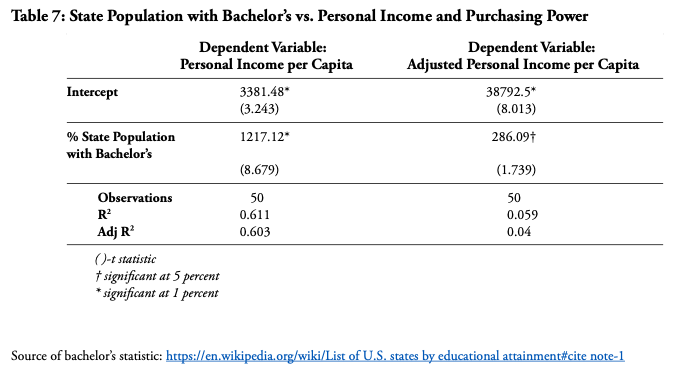
Table 7 shows the results of two single-variable regressions. In both cases, the percentage of states’ populations with a bachelor’s degree is the independent variable. In the first regression, personal income per capita is the dependent variable. It shows a strong positive (as expected) correlation between the bachelor’s variable and personal income. Not only are both the intercept and bachelor’s coefficients highly significant, the R² values are extremely high for a single-variable regression. The bachelor’s coefficient indicates that a 1-percentage-point increase in the proportion of a state’s population with a college degree is associated with a $1,217 increase in per capita income.

When personal income adjusted for states’ cost of living (purchasing power) is substituted as the dependent variable, the relationship with bachelor’s degrees essentially falls apart. The significance level of the bachelor’s coefficient falls. It indicates that a 1-percentage-point increase in the share of a state’s population with a bachelor’s is associated with less than $300 in additional purchasing power. But even this result is suspect given the vanishingly low R² values in this second regression.

The natural conclusion to draw is that states that have proportionately more bachelor’s degrees have less of an advantage than is apparent. When it comes to purchasing power, their advantage might even completely disappear. Adding control variables to the second regression would likely improve the R², but it is doubtful that the bachelor’s coefficient would maintain significance.

Net Federal Dollars vs. Personal Income

Taxes flow from states to the federal government through individually paid taxes. States then receive money back from the federal government directly through federal spending on programs like defense, Medicare, and Social Security, and less directly through state governments in programs like roads, education, and Medicaid. Because the federal government borrows, states receive more money in aggregate than they pay in. Net federal dollars is simply the ratio of what is received from the federal government versus what is paid in. Due to federal borrowing, more states’ ratios are greater than one.

Because many federal programs flow funding based on some type of determination of need, one would expect that states with lower incomes would be judged needier than those with higher incomes and would receive proportionally more federal money. Thus, in a regression with net federal dollars as the dependent variable and personal income as the independent variable, a negative relationship (fewer federal dollars as income increases) would be expected. Indeed, this is the case. Table 8 shows that both coefficients are highly significant and the personal income coefficient has the expected sign. The R² is about as good as can be expected in a single-variable regression.

As good as the regression with personal income is, a second regression reported in Table 8 is even better. It uses personal income adjusted for cost of living (purchasing power) as the independent variable. The statistical results are even stronger. Both coefficients are more significant than those in the first regression, and the R², at almost 0.4, is quite high for a single-variable regression. This indicates that relative purchasing power is playing a significant role in determining how much money states receive from the federal government.

Cost of Living vs. Policy

As explained in the body of this paper, 14 policy variables derived from a paper by economist Wayne Winegarden were initially evaluated for their impact on state-level cost of living. These variables include

1) a land-use regulation index;

2) a dummy variable for whether a state has a right-to-work law (1-does not; 0-does);

3) a dummy variable for whether a state imposes additional disability insurance requirements (1-does; 0-does not);

4) the percentage of each state’s workforce that is occupationally licensed (in decimals);

5) a grade for each state’s tort/liability system;

6) an ordinal ranking of states’ family leave requirements in excess of federal;

7) an ordinal ranking of states’ startup and filing costs associated with starting a business;

8) an ordinal ranking of states’ telecommunications regulation regimes;

9) an index of states’ energy regulation regimes (mainly electricity);

10) a measure for each state’s unemployment insurance taxation level (percentage entered in decimals);

11) each state’s minimum wage with the federal minimum wage entered as the default;

12) an ordinal ranking of each state based on the strength of a regulatory flexibility law similar to that of the federal government;

13) a dummy variable for whether a state imposes alcohol content regulation (1-does not; 0-does); and

14) a measure for each state’s workers’ compensation taxation level (a percentage but not entered as a decimal; i.e., 1 percent is entered as “1.0”).

Variables 1-4, 6, 7, 9, 11, and 12 are described (with citations) in the body of this paper. Therefore, only the remaining variables, whose statistical results are not deemed of sufficient quality to be made mention of in a policy context, are briefly described here. Citations are provided where values other than Winegarden’s ordinal rankings are used.

Tort Liability Index

The Harris Poll, for the U.S. Chamber Institute for Legal Reform, graded states’ lawsuit climates as determined by a poll of attorneys and business executives in 2015. Grades on a 100-point scale were assigned to each state, and grades ranged from West Virginia’s 46.3 to Delaware’s 76.5.^[46] Winegarden interpreted higher grades as indicators of lower-cost legal systems. One would expect a negative relationship where a higher grade (lower costs from the legal system) would be associated with a lower cost of living.

Telecommunications Regulation

Each state’s telecom regulations were evaluated on a number of dimensions. States were ranked with 1 being the least regulated and 50 being the most. More regulation is expected to result in a higher cost of living. These rankings were used in the analysis.

Unemployment Insurance

All employers are required to collect unemployment insurance (UI) taxes. This is a labor cost, and the higher it is, the higher the prices one would expect consumers to pay. This variable is expressed as a percentage of total payroll collected for UI in each state in 2015 and ranges from 0.29 percent in South Dakota to 1.53 percent in Vermont.^[47] A positive relationship between the UI and cost of living would be expected.

Regulatory Flexibility

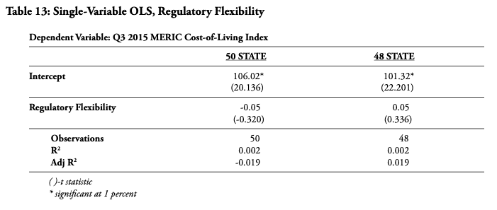
States were ranked on the basis of (1) whether they have laws similar to the federal Regulatory Flexibility Act that provide flexibility with respect to their own regulations, and (2) how large a business must be to qualify for such flexibility. A ranking of 1 indicates the greatest flexibility, while 50 indicates the least flexibility. Greater flexibility would be expected to result in lower costs, so the relationship between this ranking and the cost of living should be positive. This is true in the 48-state regression, but the results of single-variable regressions (Table 13) are so weak that this variable was excluded from the policy discussion in the body of the paper.

Alcohol Control

Some states prohibit the private sale of spirits outside of state-run or state-sanctioned stores. To the extent that this kind of regulation might impact cost of living, one would expect that states that allow for private sale would have a lower cost of living through the elimination of monopolistic pricing power in alcohol.

Workers’ Compensation

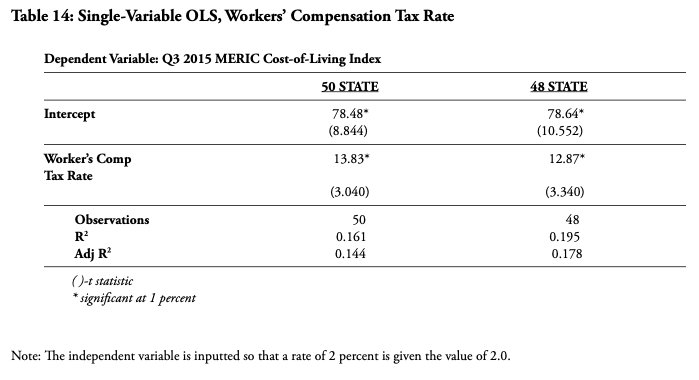
Every state has a workers’ compensation system whereby employers are taxed and employees hurt on the job are compensated from a special fund. The Oregon Department of Consumer Business Services periodically compiles an index of workers’ compensation tax costs for all the states, and 2014 values were used for this analysis.^[48] The higher the tax rate, the higher business costs are and the higher the cost of living is expected to be, so a positive relationship would be expected.

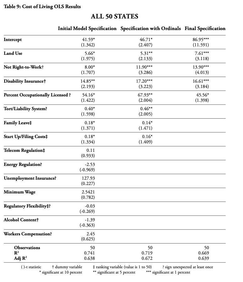
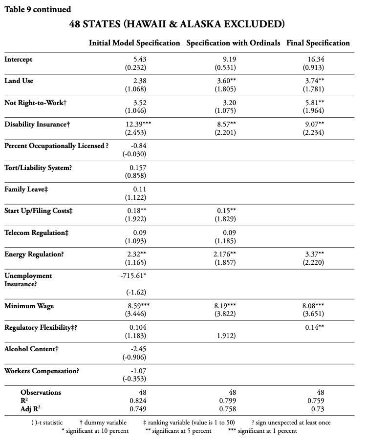
The results of six regressions are reported in Table 9. The first three regressions use observations from all 50 states. The rest use observations from only the contiguous 48 states, thereby excluding Alaska and Hawaii. Although Hawaii’s cost-of-living index value is not as much of an outlier in the third quarter of 2015 as it is in the first quarter of 2017, it is still high, along with its land-use-regulation index value. However, excluding only Hawaii as an outlier makes little intellectual sense, so it was decided to also exclude Alaska as the only other state detached from the 48. It is also an outlier in some ways, although its explanatory parameters push in directions both in concert with and opposite Hawaii’s. In both cases, initial regressions included all 14 policy variables, and insignificant variables were systematically excluded to determine two “best-fit” regressions: one that includes ordinal variables and one that does not. Ordinal variables have a tendency to bias results, although the impact of this bias appears mainly to manifest itself in the 48-state regressions. Significant results from the last four regression specifications (two 50-state regressions and two 48-state regressions) are reported in the body of this paper.

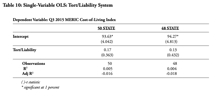
The tort/liability system variable returns an unexpected positive and significant result in the 50-state regressions, and a positive but insignificant result in the 48-state regression. Ultimately, it was decided not to include the tort/liability in the final 50-state regression because it seems clear that the variable is interacting with other variables in some sort of collinear relationship. Both 50-state and 48-state regressions using tort/liability as the only explanatory variable showed it to have no statistical significance whatsoever (Table 10). Using a different legal system measure from the Cato Institute did return negative coefficients in single-variable regressions, but they were also statistically insignificant.^[49] This indicates that state-level legal-system indexes do little to indicate legal system costs and might need refinement.

The telecom regulation result in the 48-state regression is not significant but is reported because the t-value is greater than that of the right-to-work variable, which is significant in the final 48-state regression that excludes ordinal variables. The telecom result is at least positive, as expected, but its statistical insignificance merits its exclusion from policy suggestions.

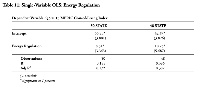
Even though the energy regulation variable returned a negative coefficient in the first 50-state regression, opposite the sign anticipated, it returned expected results in the 48-state regression. In addition, single-variable 50-state and 48-state regressions (Table 11) both yielded significant coefficients, and the fit in the 48-state regression was remarkably good.

In the initial 50-state regression, the unemployment insurance tax rate variable (UI) returned an insignificant but expectedly positive coefficient, but in the 48-state initial regression, the unexpectedly negative coefficient was significant at the 5 percent level. In the second case it was excluded from additional regressions for two reasons. First, the result is nonintuitive and second, in a 48-state single regression, the result was a positive coefficient (Table 12). Collinearity appears to be a problem.

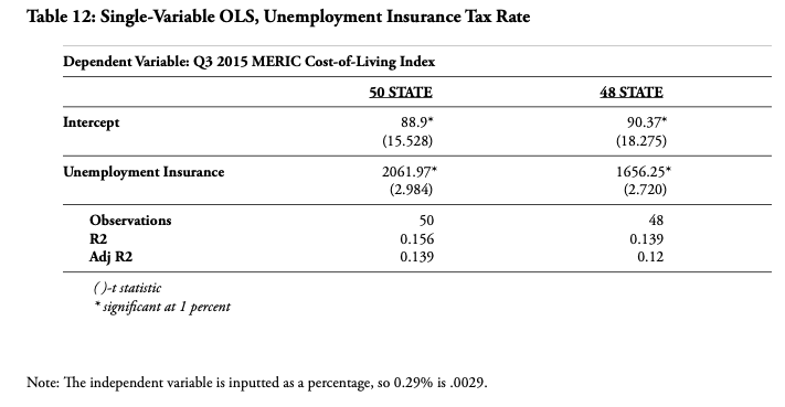
Note: The independent variable is inputted as a percentage, so 0.29% is .0029.

The regulatory flexibility variable suffers statistically from being ordinal. Depending on the set of states for the regression, it returns different results. Even though it returns significant results in the initial 48-state regression, these are ultimately rejected due to very weak single-variable regression results. Clearly, there is some unexplained collinear interaction with other variables.

The workers’ compensation tax rate variable returned opposite signs in the initial regressions with an unexpected negative sign in the 48-state regression. Nevertheless, in both single-variable regressions (Table 14), the expected sign results and the statistical results are also fairly strong. Workers’ compensation tax rates likely impact the cost of living, but the weak results in the larger regressions are cause for leaving this variable out of the policy discussion above.

________________________

Notes

1. The author worked for a state representative in Texas as a legislative aide during most of the nine years from 1994 through 2003. ↑
2. 2017 KidsCount Data Book: State Trends in Child Well-Being (Baltimore, MD: Anne E. Casey Foundation), http://www.aecf.org/m/resourcedoc/aecf-2017kidscountdatabook.pdf; “The Facts About Oklahoma Education,” Oklahoma Education Coalition, http://www.okedcoalition.org/get-the-facts.html; Admin, “8 Key Facts about Education Funding in Oklahoma (#Betterok Budget Bootcamp),” Together Oklahoma, January 22, 2017, http://togetherok.org/8-key-facts-education-funding-oklahoma-betterok-budget-bootcamp/; “Medicaid Capped Funding: Findings and Implications for Oklahomans,” State Health Reform Assistance Network, April 5, 2017, http://www.statenetwork.org/wp-content/uploads/2017/04/OK-Fact-Sheet_rev-4.4.17.pdf. ↑
3. Mississippi’s students score higher on NAEP than Michigan’s, California’s and Hawaii’s (Matthew M. Chingos and Kristin Blagg, “How Do States Really Stack Up on the 2015 NAEP?” EducationNext, October 29, 2015, http://educationnext.org/how-do-states-really-stack-up-on-the-2015-naep/). Twelve states have worse roads than Mississippi’s by one ranking’s judgment (Steven Peters, “States With the Worst Roads,” 24/7 WallSt., October 21, 2016, http://247wallst.com/special-report/2016/10/21/states-with-the-worst-roads/9/), and 16 states spend less on healthcare than Mississippi (“Health Care Expenditures Per Capita by State of Residence,” KFF.org, http://www.kff.org/other/state-indicator/health-spending-per-capita/). ↑
4. Thomas C. Frohlich, Michael Be Sauter, and Samuel Stebbing, “America’s Richest (and Poorest) States,” 24/7 Wall St., September 15, 2016, http://247wallst.com/special-report/2016/09/15/americas-richest-and-poorest-states-4/2/. ↑
5. A Google search for “cost of living calculator” yields almost 4 million results, and the first page of results, except for one selection, were various calculators, mostly aimed at cities. ↑
6. For more on price indexes, see Michael J. Boskin, “Consumer Price Indexes,” Concise Encyclopedia of Economics, 2nd ed., Library of Economics and Liberty, http://www.econlib.org/library/Enc/ConsumerPriceIndexes.html. ↑
7. For a given state, a value in Table 3 is calculated as follows: (Value in Table 1)/(Value in Table 2)/100). For Ohio, the calculation is 45,734/(92.7/100) = 49,335. ↑
8. Kiran Dhillon, “Blue States Barack Obama Won in 2012 Are More Educated Than Red States,” Time, May 15, 2014, http://time.com/101697/blue-states-barack-obama-won-in-2012-are-more-educated-than-red-states/. ↑
9. Byron Schlomach, “Oklahoma’s Teacher Pay: 30^th, Not 48^th,” Policy Analysis, 1889 Institute, August 2016, http://nebula.wsimg.com/39fac99aa2149b53f35a3140dd30a888?AccessKeyId=CB55D82B5028ABD8BF94&disposition=0&alloworigin=1. ↑
10. Jonathan Lansner, “Blue States Rank Better Than Red in Livability: What Does That Mean?” Mercury News, March 8, 2017, http://www.mercurynews.com/2017/03/08/blue-states-rank-better-than-red-in-livability-what-does-that-mean/Kevin Baker, “BlueExit: A Modest Proposal for Separating Blue States from Red,” New Republic, March 9, 2017, https://newrepublic.com/article/140948/bluexit-blue-states-exit-trump-red-america. ↑
11. “U.S. Federal Poverty Guidelines Used to Determine Financial Eligibility for Certain Federal Programs,” U.S Department of Health & Human Services, https://aspe.hhs.gov/poverty-guidelines. ↑
12. The difference averages expressed here appear to be incorrect since $29,613 – $24,600 = $5,013 and $23,334 – $23,334 – $24,600 = -$1,266. However, Alaska’s and Hawaii’s actual FPLs are higher than $24,600. Thus, the discrepancy since differences were averaged. ↑
13. R.A., “Thomas Piketty’s ‘Capital,’ Summarised in Four Paragraphs,” The Economist Explains (blog), The Economist, May 5, 2014, https://www.economist.com/blogs/economist-explains/2014/05/economist-explains. ↑
14. Michael Tanner, “Five Myths About Economic Inequality in America,” Policy Analysis 797, Cato Institute, September 7, 2016, 2, https://object.cato.org/sites/cato.org/files/pubs/pdf/pa797_2.pdf. ↑
15. Robert B. Reich, How to Shrink Inequality (blog), May 12, 2014, http://robertreich.org/post/85532751265. ↑
16. Others have pointed this out, and there is empirical evidence of this statement’s accuracy. See Enrico Moretti, “Poverty, Inequality and Cost of Living Differences,” University of Kentucky Center for Poverty Research, Discussion Paper 2010-07, August 2010, http://uknowledge.uky.edu/cgi/viewcontent.cgi?article=1055&context=ukcpr_papers.The same issue has been identified in China; see Chao Li and John Gibson, “Spatial Price Differences and Inequality in China: Housing Market Evidence” (working paper, Hamilton, New Zealand University of Waikato, March 2013), http://researchcommons.waikato.ac.nz/handle/10289/7670. ↑
17. Courtney A. Collins, “Poverty Rates, Demographics, and Economic Freedom Across America: A Comparison of Nationwide Poverty Measures,” Texas Public Policy Foundation, August 2017, https://www.texaspolicy.com/content/detail/poverty-rates-demographics-and-economic-freedom-across-america. ↑
18. Hedonic prices are essentially the differences in actual prices that reflect the value people place on external factors such as weather, with differentials likely caused by higher demand for goods and services in locations with highly desirable characteristics. ↑
19. Kevin Neels, “Determinants of Spatial Variations in the Cost of Living” (unpublished manuscript, Defense Technical Information Center, U.S. Department of Defense, October 1979), http://www.dtic.mil/dtic/tr/fulltext/u2/a095455.pdf. ↑
20. Richard J. Cebula and Michael Toma, “An Empirical Analysis of Determinants of Interstate Living-Cost Differentials, 2005,” The Journal of Regional Analysis and Policy 38, no. 3 (2008): 222-228, http://ageconsearch.umn.edu/bitstream/133000/2/08-3-2.pdf. ↑
21. Richard J. Cebula and Michael Toma, “Determinants of Interstate Differentials in the Cost of Housing, 2006,” Applied Economics Letters 17, no. 2 (2010): 153-157, http://www.tandfonline.com/doi/abs/10.1080/13504850701719900?journalCode=rael20.A problem with the last two studies is that some of the factors statistically identified with interstate differences in cost of living seem contrived to produce a result. Recall that per capita personal income is highly correlated with cost of living (see above). Cebula and Toma view cost of living as partly a function of income with higher incomes pushing up demand and prices. However, cost of living could be high for entirely different reasons, causing an area to mainly be inhabited by people with high incomes. Those with high incomes, able to afford costly and restrictive policies, could also push up the cost of living by impacting the supply of housing as well as other goods and services.The coastal-area variable Cebula and Toma describe (coast length divided by total state area), which is associated with a higher cost of living, is naturally higher for northeastern and western states, but only by an accident of history. These states tend to have higher costs of living. But coastlines also mean ports, which should produce a lower cost of living. Toxic chemical releases also reflect data bias because oil states, which are southern and tend to have lower costs of living, tend to see greater toxic releases. Yet demand for residency in southern states has been strong for many years, as indicated by net migration rates. Cebula and Toma’s single nod to policy is whether a state has a right-to-work law. ↑
22. Wayne Winegarden, “The 50-State Small Business Regulation Index,” Pacific Research Institute, July 2015, https://www.pacificresearch.org/fileadmin/images/Studies_2015/SmBusinessIndex_UpdatedVersion2_web.pdf. ↑
23. Only one of these indexes, having to do with energy regulation, was devised by Winegarden. The others were devised independently and merely compiled and converted to ordinal rankings for Winegarden’s study. Several other variables reflect binary policy options, such as whether a state has a right-to-work law or not. Others, such as specific tax levels or state minimum wages, are straightforward policy variables.Winegarden only reports ordinal rankings in his paper. Where actual values could be found, they were used in the analysis. In the case of licensing, a simplified measure compared to the index Winegarden references is used. Several of the indexes he references could not be located, so the ordinal rankings were initially included in the analysis discussed in this paper (more detail of the statistical analysis is in the appendix). Citations for various policy variables are provided where they are discussed in more detail below and in the appendix. ↑
24. It should be noted that regression analysis does require judgment and is not nearly as cut-and-dried as many pretend. Economists are notorious for using economic models whose parameters were estimated in a linear regression. Stating confidently that a government project such as a stadium will result in so many jobs and added economic activity as a result of using a mathematical model filled with coefficients pulled from dozens of studies, often with weak results (which are too often not replicable), is neither scientific nor wise. ↑
25. Joseph Gyourko, Albert Saiz, and Anita A. Summers, “A New Measure of the Local Regulatory Environment for Housing Markets: The Wharton Residential Land Use Regulatory Index,” Urban Studies 45, no. 3 (March 1, 2008): 693-729, http://real.wharton.upenn.edu/~gyourko/WRLURI/The%20Wharton%20Zoning%20Regulation%20Index-July%202,%202007.pdf ↑
26. Paul Emrath, “Government Regulation in the Price of a New Home” (National Association of Home Builders, Washington, DC, May 2, 2016), https://www.nahbclassic.org/generic.aspx?sectionID=734&genericContentID=250611&channelID=311. ↑
27. See Levin v. City & Cty. of San Francisco, 71 F. Supp. 3d 1072, 1084 (N.D. Cal. 2014). ↑
28. For an example, see Diana Baldwin, “Edmond Neighbors Upset After Golf Course Closes,” Oklahoman, January 18, 2017, http://newsok.com/article/5534772. ↑
29. Randal O’Toole, American Nightmare: How Government Undermines the Dream of Homeownership (Washington, DC: Cato Institute, 2012). ↑
30. Christina Sandefur and Timothy Sandefur, “The Property Ownership Fairness Act,” Goldwater Institute, Policy Paper, February 8, 2016, https://goldwater-media.s3.amazonaws.com/cms_page_media/2016/2/9/Final%20Property%20Rights%20paper.pdf. ↑
31. Gyourko, “A New Measure of the Local Regulatory Environment for Housing Markets,” 4. ↑
32. Gyourko, “A New Measure of the Local Regulatory Environment for Housing Markets,” 6. ↑
33. Morris M. Kleiner, “Reforming Occupational Licensing Policies,” Brookings Institution, Discussion Paper 2015-01, March 2015, https://www.brookings.edu/wp-content/uploads/2016/06/THP_KleinerDiscPaper_final.pdf. ↑
34. Winegarden describes a more complex index used for his rankings, but it could not be located. ↑
35. Byron Schlomach and Baylee Butler, “Funeral Director and Embalmer Licensure in Oklahoma,” 1889 Institute, Policy Paper, June 2017, http://nebula.wsimg.com/09e71b3950f2f349a51185bda6fa2ce3?AccessKeyId=CB55D82B5028ABD8BF94&disposition=0&alloworigin=1. ↑
36. Byron Schlomach, “The Need to Review and Reform Occupational Licensing in Oklahoma,” 1889 Institute, Policy Analysis, September 2016, http://nebula.wsimg.com/b845ef32a491f4a35fb2ef7c97b05704?AccessKeyId=CB55D82B5028ABD8BF94&disposition=0&alloworigin=1. ↑
37. Schlomach, “The Need to Review and Reform Occupational Licensing.” ↑
38. Clint Bolick, “Right to Earn a Living Act,” Goldwater Institute, Policy Paper,, https://goldwater-media.s3.amazonaws.com/cms_page_media/2016/1/5/Gi%20Right%20to%20Earn%20PDF.pdf. ↑
39. Starlee Coleman, “Arizona Becomes First State in Country to Protect the Right to Earn a Living,” press release, Goldwater Institute, April 6, 2017, http://www.goldwaterinstitute.org/en/work/topics/free-enterprise/regulations/arizona-becomes-first-state-in-country-to-protect-/. ↑
40. “Right to Work States,” National Right to Work Legal Defense Foundation, updated February 2017, http://www.nrtw.org/right-to-work-states. ↑
41. “Minimum Wage Rates for 2015, by State,” Small Business Employee Benefits and HR Blog, ZaneBenefits.com, January 7, 2015, https://www.zanebenefits.com/blog/minimum-wage-rates-for-2015-by-state. ↑
42. “State Minimum Wages/2017 Minimum Wage by State,” National Conference of State Legislatures, January 5, 2017, http://www.ncsl.org/research/labor-and-employment/state-minimum-wage-chart.aspx. ↑
43. Wayne Winegarden and Marc A. Milles, “The 50 State Index of Energy Regulation,” Pacific Research Institute, July 2014, https://www.pacificresearch.org/fileadmin/documents/Studies/PDFs/2013-2015/50States_ExecSumm8pg_Finalwebl.pdf. ↑
44. Carl Johnston and Lynne Kiesling, “Turning on the Lights 2011: The Consumer Benefits of Electric Power Competition,” National Center for Policy Analysis, Policy Report No. 332, April 2011, http://www.ncpa.org/pdfs/st332.pdf. ↑
45. Excerpt from “The New Colussus” by Emma Lazarus, engraved on a bronze plaque and affixed to the interior of the pedestal of the Statue of Liberty. ↑
46. “Lawsuit Climate Survey: Ranking the States; A Survey of the Fairness and Reasonableness of State Liability Systems,” U.S. Chamber Institute for Legal Reform (conducted by Harris Poll), September 2015, http://www.instituteforlegalreform.com/uploads/sites/1/ILR15077-HarrisReport_BF2.pdf. ↑
47. “Employer Contribution Rates: Calendar Year 2015,” U.S. Department of Labor, Employment and Training Administration, https://oui.doleta.gov/unemploy/docs/aetr-2015est.pdf. ↑
48. Robert Wilson, “2014 Oregon Workers’ Compensation Premium Rate Ranking: Reflection of the Past or Prediction for the Future?” WorkersCompensation.com, October 13, 2014, https://www.workerscompensation.com/news_read.php?id=19958. ↑
49. William P. Ruger and Jason Sorens, Freedom in the 50 States: An Index of Personal and Economic Freedom, 4^th ed. (Washington, DC: Cato Institute, 2016), 49, https://www.freedominthe50states.org/download/print-edition-2016.pdf. ↑